13.7: The Franck |
您所在的位置:网站首页 › franck condon › 13.7: The Franck |
13.7: The Franck
|
Franck-Condon Progressions
To understand the significance of the above formula for the FC factor, let us examine a ground and excited state potential energy surface at \(T = 0\) Kelvin. Shown below are two states separated by 8,000 cm-1 in energy. This is energy separation between the bottoms of their potential wells, but also between the respective zero-point energy levels. Let us assume that the wavenumber of the vibrational mode is 1,000 cm-1 and that the bond length is increased due to the fact that an electron is removed from a bonding orbital and placed in an anti-bonding orbital upon electronic excitation.  Figure 13.7.2
: Wavefunctions transitions for a harmonic oscillator model system with moderate displacement (S=1).
Figure 13.7.2
: Wavefunctions transitions for a harmonic oscillator model system with moderate displacement (S=1).
According to the above model for the Franck-Condon factor we would generate a "stick" spectrum (Figure 13.7.3 ) where each vibrational transition is infinitely narrow and transition can only occur when \(E = h\nu\) exactly. For example, the potential energy surfaces were given for S = 1 and the transition probability at each level is given by the sticks (black) in the figure below.  Figure 13.7.3
: Stick spectrum, dressed with Gaussians, for the moderate displacement (S=1) harmonic oscillator system from Figure 13.7.2
.
Figure 13.7.3
: Stick spectrum, dressed with Gaussians, for the moderate displacement (S=1) harmonic oscillator system from Figure 13.7.2
.
The dotted Gaussians that surround each stick give a more realistic picture of what the absorption spectrum should look like. In this first place each energy level (stick) will be given some width by the fact that the state has a finite lifetime. Such broadening is called homogeneous broadening since it affects all of the molecules in the ensemble in a similar fashion. There is also broadening due to small differences in the environment of each molecule. This type of broadening is called inhomogeneous broadening. Regardless of origin the model above was created using a Gaussian broadening The nuclear displacement between the ground and excited state determines the shape of the absorption spectrum. Let us examine both a smaller and a large excited state displacement. If \(S = ½\) and the potential energy surfaces in this case are:  Figure 13.7.4
: Wavefunctions transitions for a harmonic oscillator model system with small displacement (S=1/2).
Figure 13.7.4
: Wavefunctions transitions for a harmonic oscillator model system with small displacement (S=1/2).
For this case the "stick" spectrum has the appearance in Figure 13.7.5 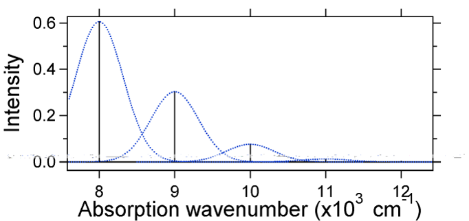 Figure 13.7.5
: Stick spectrum, dressed with Gaussians, for the small displacement (S=1/2) harmonic oscillator system from Figure 13.7.4
.
Figure 13.7.5
: Stick spectrum, dressed with Gaussians, for the small displacement (S=1/2) harmonic oscillator system from Figure 13.7.4
.
Note that the zero-zero or \(S_{0,0}\) vibrational transition is much large in the case where the displacement is small. As a general rule of thumb the \(S\) constant gives the ratio of the intensity of the \(v = 2\) transition to the \(v = 1\) transition. In this case since \(S = 0.5\), the \(v=2\) transition is 0.5 the intensity of \(v=1\) transition. As an example of a larger displacement the disposition of the potential energy surfaces for S = 2 is shown below.  Figure 13.7.6
: Wavefunctions transitions for a harmonic oscillator model system with strong displacement (S=2).
Figure 13.7.6
: Wavefunctions transitions for a harmonic oscillator model system with strong displacement (S=2).
The larger displacement results in decreased overlap of the ground state level with the v = 0 level of the excited state. The maximum intensity will be achieved in higher vibrational levels as shown in the stick spectrum. 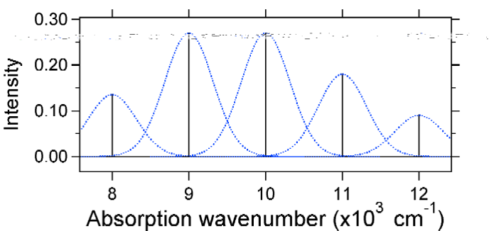 Figure 13.7.7
: Stick spectrum, dressed with Gaussians, for the large displacement (S=2) harmonic oscillator system from Figure 13.7.6
.
Figure 13.7.7
: Stick spectrum, dressed with Gaussians, for the large displacement (S=2) harmonic oscillator system from Figure 13.7.6
.
The absorption spectra plotted below all have the same integrated intensity, however their shapes are altered because of the differing extent of displacement of the excited state potential energy surface.  Figure 13.7.8
: Stick spectra, dressed with Gaussians, for the small to large displacements in harmonic oscillator system described above.
Figure 13.7.8
: Stick spectra, dressed with Gaussians, for the small to large displacements in harmonic oscillator system described above.
So the nature of the relative vibronic band intensities can tell us whether there is a displacement of the equilibrium nuclear coordinate that accompanied a transition. When will there be an increase in bond length (i.e., \(Q_e > R_e\))? This occurs when an electron is promoted from a bonding molecular orbital to a non-bonding or anti-bonding molecular orbitals (i.e., when the bond order is less in the excited state than the ground state). Non-bonding molecular orbital \(\rightarrow\) bonding molecular orbital Anti-bonding molecular orbital \(\rightarrow\) bonding molecular orbital Anti-bonding molecular orbital \(\rightarrow\) non-bonding molecular orbitalIn short, when the bond order is lower in the excited state than in the ground state, then \(Q_e > R_e\); an increase in bondlength will occur when this happens. |
【本文地址】
今日新闻 |
推荐新闻 |